TDA in a nutshell: how can we find multidimensional voids and explore the “black boxes” of deep learning?

Topological Data Analysis (TDA) is an innovative set of techniques that is gaining an increasing relevance in data analytics and visualization. It uses notions of a miscellaneous set of scientific fields such as algebraic topology, computer science and statistics.

Its resulting tools allow to infer relevant and robust features of high-dimensional complex datasets that can present rich structures potentially corrupted by noise and incompleteness[74].

Here, two of the most common TDA methodologies will be briefly and intuitively introduced along with some of their interesting applications. 

• Topological Data Compression to represent the shape of data
• Topological Data Completion to “measure” the shape of data

Topological Data Compression

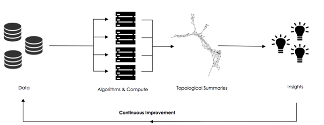
Topological Data Compression algorithms aim at representing a collection of high dimensional clouds of points through graphs. These techniques rely on the fact that an object made of lots or infinitely many points, like a complete circle, can be approximated using only some nodes and edges [28].

The premise underlying TDA is that shape matters and in general real data in high dimensions is nearly always sparse, and tends to have relevant low dimensional features.

Consider for example the “Y”-shape detectable in the figure below

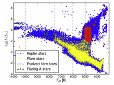
This shape occurs frequently in real data sets. It might represent a situation where the core corresponds to the most frequent behaviours and the tips of the flares to the extreme ones [30]. However, classical models such as linear ones and clustering methods cannot detect satisfactorily this feature.

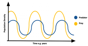
Another not trivial but important shape is the circular one; in fact loops can denote periodic behaviours. For example, in the Predatory-Prey model in the figure below, the circular shapes are due to the periodicity of the described biological system.

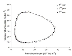
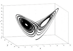
In a dynamic system, an attractor is a set towards which it tends to evolve after a sufficiently long time. System values that get close enough to the attractor ones have to remain close to them, even if slightly disturbed. A trajectory of a dynamic system on an attractor must not satisfy any particular property, but it is not unusual for it to be periodic and to present loops.

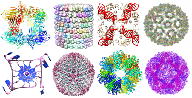
Consider, moreover, the great amount of not trivial geometric information carried by biomolecules and their importance for the analysis of their stability [63].

But, how can we go from an highly complex set of data points (PCD) to a simple summary of their main features and relations?

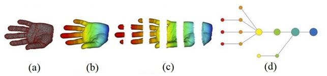
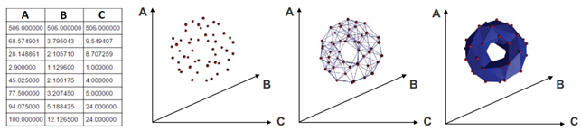
Topological Data Compression can detect these shapes easily and the main algorithm in this area is the Mapper. Its steps can be described as follows[88].

1. A PCD representing a shape is given. 
2. It is covered with overlapping intervals by coloring the shape using filter values. 
3. It is broken into overlapping bins. 
4. The points in each bin are collapsed into clusters. Then a network is built representing each cluster by a vertex and drawing an edge when clusters intersect.

In work published in 2011 by Nicolau, Carlsson, and Levine[37], a new subtype of breast cancer was discovered[95] using the Progression Analysis of Disease (PAD), an application of the Mapper that provided an clear representation of the dataset. The used dataset describes the gene expression profiles of 295 breast cancer tumours [5]. It has 24.479 attributes and each of them specifies the level of expression of one gene in a tissue sample of the corresponding tumour. The researchers discovered the three-tendril “Y”-shaped structure shown below.

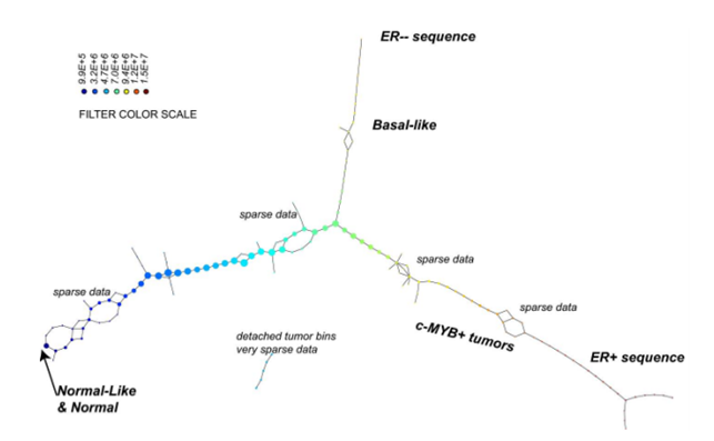
In addition, they found that one of these tendrils decomposes further into three clusters. One of these three clusters corresponds to a distinct new subtype of breast cancer that they named c-MYB+. A standard approach to the classification of breast cancers, based on clustering, divides breast cancers into five groups and these results suggested a different taxonomy not accounted before. In particular, the dendrogram of this dataset is shown below (the bins defining the c-MYB+ group are marked in red).

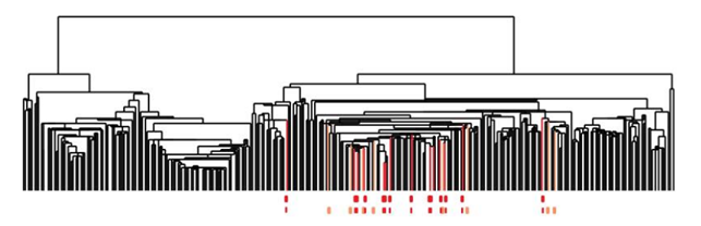
The c-MYB+ tumors are scattered among different clusters and there are many non-members of their group that lie in the same high-level cluster. Although, PAD was able to extract this group that turns out to be both statistically and clinically coherent. The new discovered subtype of cancer exhibits a 100% survival rate and no metastasis indeed. No supervised step beyond distinction between tumour and healthy patients was used to identify this subtype. The group has a clear, distinct and statistically significant molecular signature, this highlights coherent biology that is invisible to cluster methods. The problem is that clustering breaks data sets into pieces, so it can break things that belong together apart.

Improved Machine Learning Algorithms Ayasdi[7] is a machine intelligence software company that offers to organizations solutions able to analyse data and to build predictive models from them[9].  In particular, the Ayasdi system runs many different unsupervised and supervised machine learning algorithms on data, finds and ranks best fits automatically and then applies TDA to find similar groups in the results. 

This is performed to reduce the possibility of missing critical insights by reducing the dependency on machine learning experts choosing the right algorithms [10]. This methodology has lead to many achievements, for example:

• DARPA (Defense Advanced Research Projects Agency) used Ayasdi Core to analyse acoustic data tracks. The analysis identified signals that had been previously classified from traditional signal processing methods as unstructured noise [9].
• Using TDA on the portfolio of a G-SIB institution, the bank was able to identify performance improvements by 103bp in less than two weeks. This was worth over 34 million annually, despite this portfolio had been heavily analysed previously [26].
• TDA was used on the care process model for pneumonia of the Flagler Hospital. This methodology could extract nine potential pneumonia care pathways, each with distinctive elements. This represented a potential savings of more than $400K while delivering better care [6].

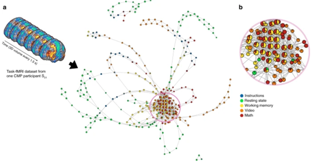
TDA-based data-driven discovery has great potential application for decision-support for basic research and clinical problems such as outcome assessment, neuro-critical care, treatment planning and rapid, precision-diagnosis [2]. For example, it has revealed new insights of the dynamical organization of the brain.

As Manish Saggar reports [1]

“How our brain dynamically adapts to perform different tasks is vital to understanding the neural basis of cognition. Understanding the brain’s dynamical organization is crucial for finding causes, cures and effective treatments for neurobiological disorders. The brain’s inability to dynamically adjust to environmental demands and aberrant brain dynamics have been previously associated with disorders such as schizophrenia, depression, attention deficiency and anxiety disorders. However, the high spatiotemporal dimensionality and complexity of neuroimaging data make the study of whole-brain dynamics a challenging endeavor.”

The scientists using TDA have been able to collapse data in space or time and generate graphical representations of how the brain navigates through different functional configurations. This revealed the temporal arrangement of whole-brain activation maps as a hybrid of two mesoscale structures, i.e., community and core−periphery organization.

Remarkably, the community structure has been found to be essential for the overall task performance, while the core−periphery arrangement revealed that brain activity patterns during evoked tasks were aggregated as a core while patterns during resting state were located in the periphery.

TDA has been used also for improving and better understating ML and AI algorithms. Neural Networks are powerful but complex and opaque tools. Using Topological Data Analysis, we can describe the functioning and learning of a convolutional neural network in a compact and understandable way. In paper [3] the researchers explain how deep neural networks (DNN) are trained using a gradient descent back propagation technique which trains weights in each layer for the sole goal of minimizing training error. Hence, the resulting weights cannot be directly explained. 

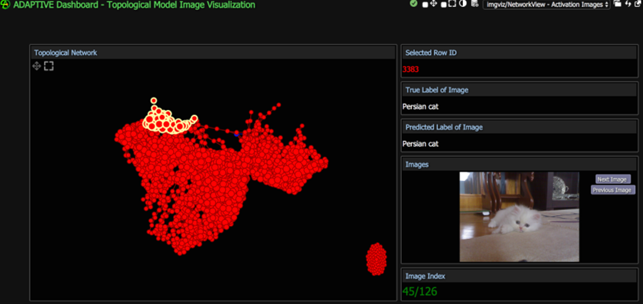
Using TDA they could extract useful insights on how the neural network they were using was thinking, specifically by analysing the activation values of validation images as they pass through each layer.

Below you can see as they have developed an Adaptive Dashboard visualization that allowed them to select and view groups of nodes in a topological model.

They reported

“Instead of making assumptions about what the neural network may be focusing on, suppose we had a way of knowing exactly which areas on the image were producing the highest activation values. We can do such analysis with the use of heat maps”

“(…) the pink colored spots are the locations where the neural network gave relatively high activations at nodes. So we can infer that VGG16 was focusing on the cat’s eyes and stripes when classifying this picture.

(…)So far we showed how to use TDA to identify clusters of correct and incorrect classifications. When we built the model using the activation values at several layers, we noticed that the misclassifications clustered into a single dense area. It is more interesting to analyze multiple clusters for which the reason for poor classification is different for each one.

(…)We converted 2,000 randomly picked images and extracted 5,000 pixel features. In this model, the images represented a majority of the 1,000 possible ImageNet labels. Each of the test images was also given an extra one-hot feature for being ”problematic”. We defined a problematic label to be one that we encountered at least three times in the test set and had an overall accuracy of less than 40%.

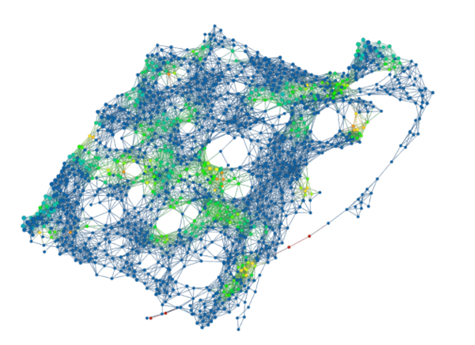
The topological model below is coloured by the density of problematic labels. The green nodes contain quite a few images that had problematic labels while blue nodes had almost none. The images with problematic labels cluster into roughly 4 distinct areas.

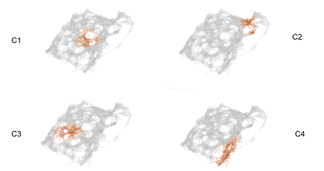
“The category of pictures in Cluster 1 were ordinary pictures with cluttered or unusual backgrounds. (…)Cluster 2 consists of images that are shiny or have glare. These types of images could have been rare in the training set so VGG16 automatically associates glare to a small set of classes. (…)Cluster 3 contains several chameleons (…) that have falsely been labelled as green lizards. This is likely because chameleons tend to blend in with their backgrounds similarly to how these green lizards blend in with the leafy environment. We can infer that there were few pictures of chameleons in the training set with green colored backgrounds. (…)In Cluster 4 we run into images with shadows and very low saturations. Here VGG16 faults when its identification of certain objects relies on color. We get false identifications when there is confusion caused by shadows and lack of color.”

The researcher concludes

“When we are able to identify unique clusters of incorrect classifications like in this example, we can then train new learners to perform well on each of these clusters. We would know to rely on this new learner when we detect that a test image exhibits similar features as the cluster’s topological group. In this case, the features were the pixel data of the images but we believe that the same methods would apply when analyzing the activation values as well. (…)With this new information on how the algorithm performs, we can potentially improve how we make predictions. We can find multiple clusters of images that make misclassifications for different reasons. Our next step would be to train new learners to perform well on the specific clusters that misclassify for certain reasons.”

Topological Data Completion

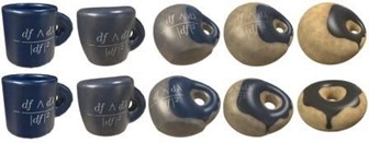
Topological data completion aims at detecting and counting properties of the shape of data that are preserved under continuous deformations such as crumpling, stretching, bending and twisting, but not gluing or tearing. Below, you can see a the figure that makes you understand the well-known mathematical joke “a topologist is a person who cannot tell the difference between a coffee mug and a donut”.

Single components, loops and voids are examples of these invariant properties and they are called Betti-0, Betti-1 and Betti-2, respectively. Below you can see Betti numbers of some shapes. For the torus, two auxiliary rings are added to explain Betti-1= 2 [34].

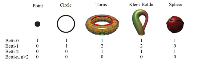
A Betti-n with a n>2 describes a “void” in higher dimensions, a multidimensional hole. In order to better understand higher dimensions you can start with the 4th watching the video below or directly playing the videogame “Miegakure: Explaining the Fourth Dimension”.

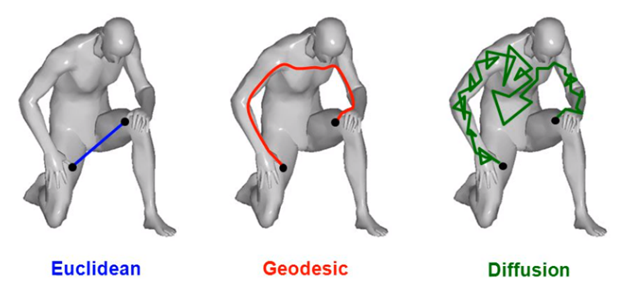
Now that we know what topologists look for, we need to have an idea of how they see “distances”. Without diving into mathematical technicalities, you can see below some distinct ways of considering distances between two points [19].

Now we can briefly describe the basic steps of topological data completion. We start by getting an input that is a finite set of elements coming with a notion of distance between them. The elements are mapped into a point cloud (PCD). Then this PCD is completed by building “continuous” shape on it, called a complex.

However, there are many ways to build complexes from a topological space. For example, which value of d should we use below to decide that two points are “close” one another?

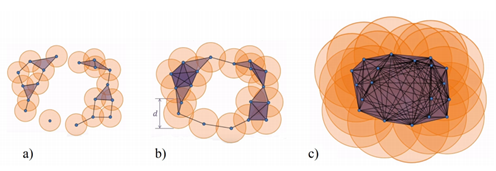
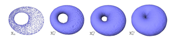
You don’t have to choose, you can consider all the (positive) distances d! Note that each hole appears at a particular value d1, and disappears at another value d2>d1.  Below another example: a PCD sampled on the surface of a torus and its offsets for different values of the radius r. For r1 and r2, the offsets are “equivalent” to a torus, for r3 to a sphere [48].

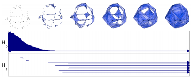
Given a parameterized family of spaces, the topological features that persist over a significant parameter range are to be considered as true features with short-lived characteristics due to noise [70]. 

We can represent the persistence of the hole with a segment [d1,d2).  In the figure below, H0 represents the persistence (while d grows) of Betti-0 (single components), while H1 the one of Betti-1 (circles).

Using this approach we can associate to a set of points with a notion of distance a persistence diagram as the one shown above that represents its topological fingerprint. For example, below you can see the topological fingerprints of the icosahedron (a) and fullerene C70 (b). They are shown respectively in (c) and (d) where there are three panels corresponding to β0, β1 and β2 bars, respectively [123].

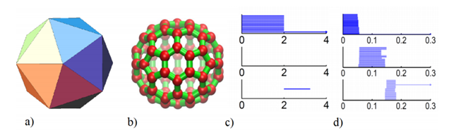
Note that for the icosahedron: 

• β0: Originally 12 bars coexist, indicating 12 isolated vertices. Then, 11 of them disappear simultaneously with only one survived. These vertices connect with each other at ε = 2A˚, i.e., the designed bond length. The positions where the bars terminate are exactly the corresponding bond lengths. 

• β1: As no one-dimensional circle has ever formed, no circle is generated. 

• β2: There is a single bar, which represents a two-dimensional void enclosed by the surface of the icosahedron. 

In regarding of the fullerene C70 barcodes: 

• β0: There are 70 initial bars and 6 distinct groups of bars due to the presence of 6 types of bond lengths in the C70 structure. 

• β1: There is a total of 36 bars corresponding to 12 pentagon rings and 25 hexagon rings. It appears that one ring is not accounted because any individual ring can be represented as the linear combination of all other rings. Note that there are 6 types of rings. 

• β2: 25 hexagon rings further evolve to two-dimensional holes, which are represented by 25 bars. The central void structure is captured by the persisting β2 bar.

These studies have been used in a wide range of applications, below some examples are reported. 

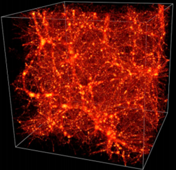
In [17] and [51], this technique has been used to provide a substantial extension of available topological information about the structure of the Universe. Below you can see the Cosmic Web in an LCDM simulation [17]. 

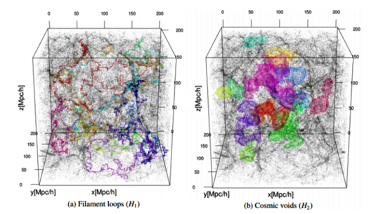
While connencted components, loops and voids do not fully quantify topology, they extend the information beyond conventional cosmological studies of topology in terms of genus and Euler characteristic [17]. Below you can see filament loops (a) and voids (b) identified in the Libeskind et al. (2018) dataset using SCHU. The most significant 10 filament loops (a) and the most significant 15 cosmic voids generators (b) are shown in different colours [51].

TDA has been used to find significant features hidden in a large data set of pixelated natural images (3×3 and 5×5 high-contrast patches). 

The subspace of linear and quadratic gradient patches forms a dense subset inside the space of all high-contrast patches and it was found to be topologically equivalent to the Klein bottle, a mathematical object that lives in 4-dimensions. 

We represent a Klein Bottle in glass by stretching the neck of a bottle through its side and joining its end to a hole in the base. Except at the side-connection (the nexus), this properly shows the shape of a 4-D Klein Bottle.

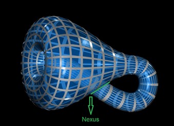
This could lead to an efficient encoding of a large portion of a natural image: instead of using an “ad hoc” dictionary for approximating high-contrast patches, one can build such a dictionary in a systematic way by generating a uniform set of samples from the ideal Klein bottle [35].

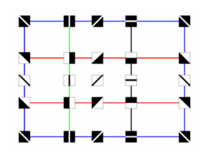
Traditionally, the structure of very complex networks has been studied through their statistical properties and metrics. However, the interpretation of functional networks can be hard. This had motivated the widespread of thresholding methods that risk overlooking the weak links importance. In order to overcome these limits efficient, alternative analysis of brain functional networks have been provided [24].

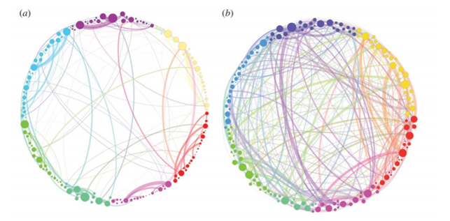
Above a simplified visualization of the results of TDA analysis on the relations of different areas of the brain. The colours represent communities obtained by modularity optimization. In (a) the placebo baseline is shown, in (b) the post-psilocybin structure one. The links widths are proportional to their weight and the diameter of the nodes to their strength [24].

These tools were applied to compare functional brain activity after intravenous infusion of placebo and psilocybin, a psychoactive component. The results, consistently with psychedelic state medical descriptions, show that the post-psilocybin homological brain structure is characterized by many transient structures of low stability and of a low number of persistent ones. This means that the psychedelic state is associated with less constrained and more inter-communicative brain activities[24].

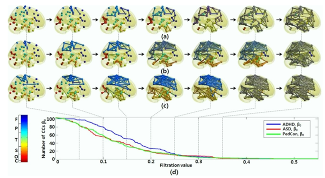
In [50], to overcome the threshold problem, TDA was used to model all brain networks generated over every possible threshold. The evolutionary changes in the number of connected components are displayed below.

In [36], TDA was successfully used to find hidden structures in experimental data associated with the V1 visual cortex of certain primates. 

In conclusion, Topological Data Analysis is a recent and fast growing branch of mathematics that has already proved to be able of providing new powerful approaches to infer robust qualitative, and quantitative, information about the structure of highly-dimensional, noisy and complex data. 

Furthermore, TDA is increasingly being used with ML and AI techniques to improve and control their processing. This is why we can now talk about TML, Topological Machine Learning. As we can read on the paper “Topology of Learning in Artificial Neural Networks”[4]:

“Understanding how neural networks learn remains one of the central challenges in machine learning research. From random at the start of training, the weights of a neural network evolve in such a way as to be able to perform a variety of tasks, like classifying images. Here we study the emergence of structure in the weights by applying methods from topological data analysis. We train simple feedforward neural networks on the MNIST dataset and monitor the evolution of the weights. When initialized to zero, the weights follow trajectories that branch off recurrently, thus generating trees that describe the growth of the effective capacity of each layer. When initialized to tiny random values, the weights evolve smoothly along two-dimensional surfaces. We show that natural coordinates on these learning surfaces correspond to important factors of variation.”

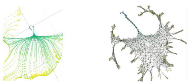
Above you can see on the left a detail of the PCA projection of the evolution of the weights for the first hidden layer. Several phases are visible: uniform evolution (blue), parallel evolution along a surface (green), chaotic evolution (yellow). On the right, the learning graph representing the surface as a densely connected grid is shown.

Sources: